
The Social Security 2100 Act: Who Wins and Who Loses?
Policy proposals such as the Social Security 2100 Act can have different effects on people depending on their age, education, family type, income, savings and many other factors.
The most common way to summarize the effects on different types of households is through a static distributional analysis. In a static distributional analysis, the effects of a policy proposal are typically shown by household income for individual years.1 This type of analysis, however, does not summarize all of the economic effects on a household over time and as economic conditions change. PWBM describes the ways in which this traditional approach to distributional analysis falls short.
To address those shortcomings and provide a measure that broadly characterizes a policy reform’s effects on households, we introduce dynamic distributional analysis using PWBM’s dynamic model. Specifically, we calculate the equivalent variation, defined in Nishiyama and Smetters (2014),2 to describe the effects of the Social Security 2100 Act on different types of households. The equivalent variation for a policy reform is the one-time payment or charge to a household that makes the household just as well off were the policy reform to be enacted. A positive equivalent variation means that the household would be better off under the policy reform; a negative equivalent variation means that the household would be worse off under the policy reform. This method allows us to analyze the policy reform’s effects across different types of households and across generations.
Table 1 summarizes the provisions in the proposal, which include increasing payroll taxes and increasing Social Security benefits. We previously showed the Act leads to a moderate drop in GDP. We found that household savings drops in response to the Act, which leads to less investment in productive capital. Less productive capital leads to a drop in wages, however, interest rates rise as the existing capital becomes more valuable.
| Current Policy (2018) | Social Security 2100 Act | |
|---|---|---|
| Benefit Provision | ||
| Primary Insurance Amount (PIA) Bend Points | 90 / 32 / 15 | 93 / 32 / 15 / 2 |
| Cost of Living Adjustment (COLA) | CPI for Urban Wage Earners and Clerical Workers (CPI-W) | CPI for Elderly (CPI-E) |
| Special Minimum PIA | Indexed to CPI-W, full special minimum PIA is $872.50 in 2019 | Minimum PIA tied to COLA. Minimum PIA set at 125% of poverty line in 2020, growing by the national Averate Wage Index (AWI) afterward |
| Tax Provision | ||
| Income Thresholds for Taxes on OASDI Benefits | Minimum income thresholds of $34,000 (single) and $44,000 (joint); up to 85% of benefits are taxable | Minimum income thresholds set at $50,000 (single) and $100,000 (joint); up to 85% of benefits are taxable |
| Payroll Taxes on Wage Earnings Above $400,000 ("Donut Hole") | No | OASDI combined employer & employee tax rate |
| OASDI Combined Employer & Employee Tax Rate | 12.4% | Increase by 0.1 percentage points annually until reaching 14.8% by 2043 |
| Other Provisions | ||
| Merge the OASI and DI trust funds | OASI and DI trust funds are separate | OASI and DI trust funds are merged |
In Table 2, we present the equivalent variation by household age and income for the Social Security 2100 Act by household age and income. Households are grouped by percentile of taxable income and reported in five-year intervals by age. We start with households who are five years from being born (and 25 years from entering the labor force at age 20) and end with households who are 95 years old when the Social Security 2100 Act is enacted. For example, our analysis shows that, on average, a 35-year-old between the 50th and 80th income percentiles has an equivalent variation of -$3,788. This value means that these households would be indifferent between being charged $3,788 and the Social Security 2100 Act becoming law.
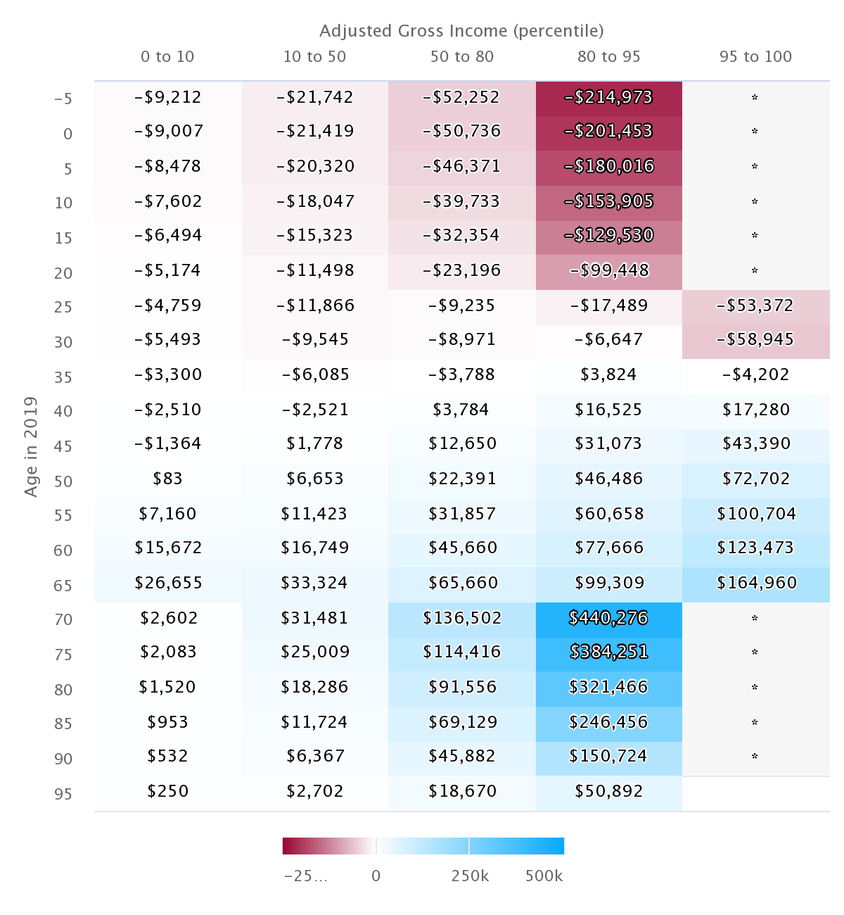
Note: Consistent with our previous dynamic analysis and the empirical evidence, the projections above assume that the U.S. economy is 40 percent open and 60 percent closed. Specifically, 40 percent of new government debt is purchased by foreigners. Asterisks indicate that the dynamic OLG model generates an insufficient number of simulated households within the age and income range to compute an equivalent variation that represents actual U.S. households with the same age and incomes.
We identify four significant distributional effects of the Social Security 2100 Act:
- People over age 45 gain from the Act because the Act increases benefits.
- In addition to the better benefits, rising interest rates provide a modest benefit for wealthier and recently retired households. Personal savings, which typically peak near retirement, provide more income as interest rates rise.
- In general, households under age 45 are worse off because of higher taxes and lower wages.
- Higher-income, younger households have the lowest equivalent variations. These younger households will end up paying higher payroll taxes, much of which comes from a new tax on income above $400,000.
Overall, this analysis shows that, if passed, the Social Security 2100 Act--which stabilizes the Social Security Trust Fund at the expense of modest economic growth--produces gains for older households while producing losses for future generations of workers, particularly high-income, younger workers. Unlike static distributional analysis, the dynamic distributional analysis of the Social Security 2100 Act captures dynamic economic effects such as the impact that lower wages and higher interest rates have on young and old households.
Written by Jon Huntley under the direction of Efraim Berkovich and Kent Smetters, with additional support and guidance from Kimberly Burham. Prepared for the PWBM website by Mariko Paulson. Calculations are based on PWBM’s model that is developed and maintained by PWBM staff.
-
For examples of static distributional analysis, see analyses by Penn Wharton Budget Model, the Joint Committee on Taxation, the Congressional Budget Office, the Tax Policy Center and the Tax Foundation. ↩
-
Nishiyama, Shinichi and Kent Smetters. "Analyzing fiscal policies in a heterogeneous-agent overlapping-generations economy." In Handbook of Computational Economics, vol. 3, pp. 117-160. Elsevier, 2014. ↩
    Age in 2019,0 to 10,10 to 50,50 to 80,80 to 95,95 to 100
    -5,-9212,-21742,-52252,-214973,
    0,-9007,-21419,-50736,-201453,
    5,-8478,-20320,-46371,-180016,
    10,-7602,-18047,-39733,-153905,
    15,-6494,-15323,-32354,-129530,
    20,-5174,-11498,-23196,-99448,
    25,-4759,-11866,-9235,-17489,-53372
    30,-5493,-9545,-8971,-6647,-58945
    35,-3300,-6085,-3788,3824,-4202
    40,-2510,-2521,3784,16525,17280
    45,-1364,1778,12650,31073,43390
    50,83,6653,22391,46486,72702
    55,7160,11423,31857,60658,100704
    60,15672,16749,45660,77666,123473
    65,26655,33324,65660,99309,164960
    70,2602,31481,136502,440276,
    75,2083,25009,114416,384251,
    80,1520,18286,91556,321466,
    85,953,11724,69129,246456,
    90,532,6367,45882,150724,
    95,250,2702,18670,50892